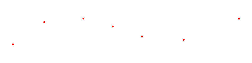
Freeform Curves:

Freeform curves are often constructed to satisfy one of three generic problems: interpolation, least squares approximation, and shape approximation. We briefly introduce each in turn.

1. Interpolation

   Informal Definition
   Given an ordered sequence of (n+1) points, possibly with associated tangent vector information, generate a curve that passes through the points in the given order, matching the provided tangent information, if any.

   1. In the simplest case, we want a single curve to interpolate a set of points.

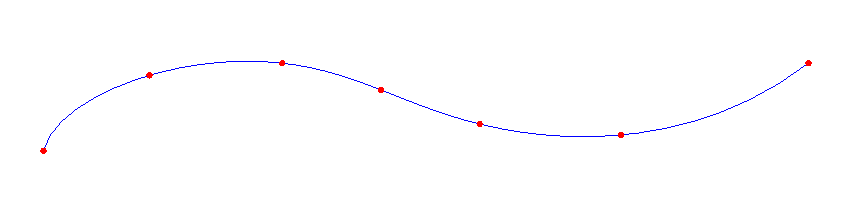
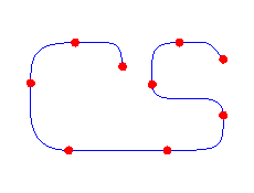
      Given a set of 7 points (i.e., n=6)	We construct a single curve that exactly interpolates them

      Notes:

      1. Creating a single curve through n+1 points requires a curve of degree n. (Hence the curve above is degree 6.)
      2. Such a curve is not unique unless additional constraints are specified. Typically this is accomplished by specifying parameter values at which the n+1 points are to be interpolated. Therefore, this version of the interpolation problem is specified more completely as:
         Given:
         • n+1 points: P₀, …, P_n
         • n+1 strictly increasing parameter values, t₀, …, t_n
         Generate the unique single polynomial curve of degree n, P(t), such that:
         P(t_i) = P_i, 0≤i≤n
   2. An alternative approach generates not one, but several pieces of different curves that, when placed end-to-end, exactly interpolate all the points in order. Such piecewise curves are called splines, and each piece of the spline is called a span (or a segment). A major advantage to the use of splines is that the polynomial degree can be fixed (degree three cubic curves are especially common) while still obtaining a piecewise curve that exactly passes through all the provided points.

      It is usually important that the spans meet "smoothly". Before discussing how that can be done, it is important to define what "smooth" means. Mathematically, we base measures on differential quantities (tangent vectors, curvature vectors, etc.). There are two common specific measures used for parametric curves: parametric continuity (C^k) and the (usually) somewhat weaker geometric continuity (G^k). The two measures are defined recursively. Specifically, given curves (or curve spans) P(t) and Q(t):

      • P and Q meet with C⁰ continuity if the end point of P is coincident with the start point of Q. They meet with C^k continuity if (i) they meet with C^k-1 continuity, and (ii) if the k-th derivative at the end of P exactly matches in length and direction the k-th derivative at the start of Q.
      • P and Q meet with G⁰ continuity if the end point of P is coincident with the start point of Q. (Same as for C⁰.) They meet with G^k continuity if (i) they meet with G^k-1 continuity, and (ii) if the unit vector in the direction of the k-th derivative at the end of P exactly matches that of the k-th derivative at the start of Q. (Note that the lengths of these two vectors need not be the same; only their direction.)

      Note that C⁰ and G⁰ are synonomous. Both require only that the end point of P is coincident with the start point of Q.

      When creating splines or other piecewise curves, we typically want smooth joins that are C¹ and/or G¹. Sometimes C² and/or G² is important; rarely is any higher level of continuity required.

      Note also that we occasionally don't want spans to meet smoothly. For example, sometimes we want to inject cusps: points along a piecewise polynomial curve that are C⁰/G⁰ but not G¹. (It turns out that cusps are often C¹!) In font design, for example, some letters require sharp corners. We will see one way to get cusps when we consider B-Splines below.

      Different schemes employ different approaches to achieve desired smoothness goals.

      Approach 1: Interpolating two or more (point, tangent) pairs

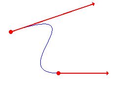
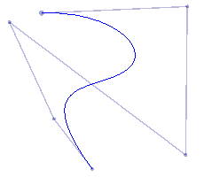
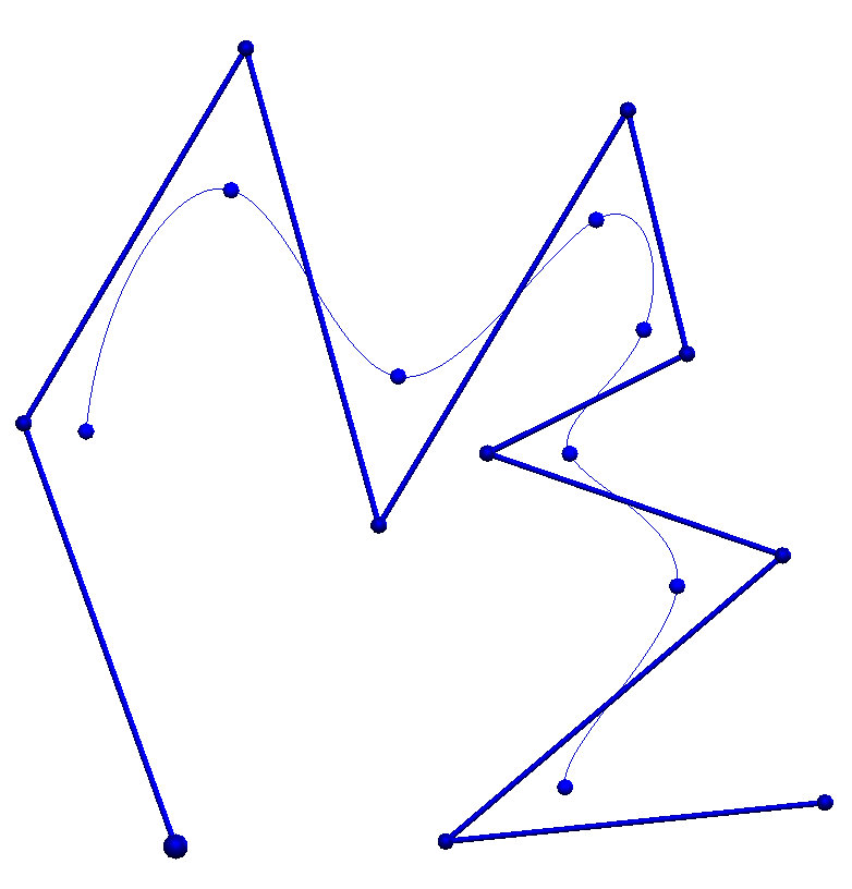
      One very direct way to achieve C¹ (or G¹) continuity is to allow the designer to associate explicit tangent vectors with each point to be interpolated. Then each span starts at point i, matching the tangent there, and ends at point (i+1), matching the tangent there. This leads to Hermite curves:

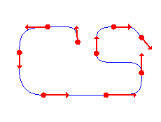
      Two (point, tangent vector) pairs and the corresponding Hermite curve	A piecewise Hermite curve built from several (point, tangent vector) pairs	The previous geometry with the vectors suppressed

      The following two examples illustrate Hermite curve construction, including a study of the effects of making the interpolated vectors very large and/or very small.

      Example 1: Single Hermite curve construction

      Example 2: Composite Hermite curve construction

      Approach 2: Interpolating collections of points without user-supplied tangents

      Associating explicit vectors with the points is an ideal way to guarantee that all spans meet smoothly, and the vectors can be a nice design handle. However requiring specification of vectors becomes an unreasonable burden on the designer when he or she simply wants a curve to be generated that passes through a given set of points. Hence most other common spline-based interpolation schemes attempt to automatically determine appropriate tangent vectors to associate with the points based strictly on the supplied point data. Two common such techniques are Catmull-Rom splines and Cardinal Splines. They differ in terms of how they use the adjacent points on a given span, and each employs a scalar parameter when doing so. The image below was created as a Catmull-Rom spline, but it could also have been generated as a Cardinal spline if the parameter were to be set appropriately.

      

2. Least Squares Curve Approximation

   Informal Definition
   Given an ordered sequence of (n+1) points and a desired polynomial degree d < n, generate a curve of degree d that minimizes the sum of the squares of the distances between the (n+1) points and the curve.

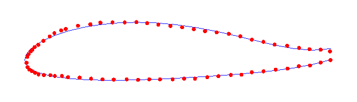
   This technique is oftentimes used in the context of digitizing a given shape because we frequently obtain a very large number of points, but a relatively small degree curve suffices to capture the essence of the shape. In the example below, we use a degree 6 curve to approximate 68 points.

   

3. Shape approximation

   Informal Definition
   Given an ordered sequence of (n+1) points, generate a curve whose shape mimics that implied by the ordered set of points.

   1. Example 1: A Bezier curve can be represented using a single polynomial of degree n, written as a function of the (n+1) points (called control points).

      A degree 5 Bezier curve	The curve with its control points	The curve with its control polygon

      Two basic properties of Bezier curves are evident in these examples:

      1. The Bezier curve starts at the first control point and stops at the last control point. (In general, it will not pass through any other control point.)
      2. The vector tangent to the Bezier curve at the start (stop) is parallel to the line connecting the first two (last two) control points.

      There are several other interesting properties of Bezier curves.

   2. As was the case with interpolation above, there are spline-based alternatives.

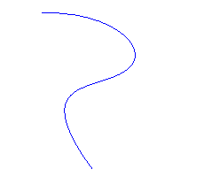
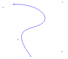
      Example 2: A B-Spline is represented as a piecewise polynomial curve – also written as a function of the (n+1) points – in which the polynomial degree, d, of the curve is decoupled from the number of control points. We are given (n+1) control points, and we say the B-Spline is of order, k = (d+1). The figure below, for example, shows a cubic (k=4; d=3) B-Spline defined using 10 control points (n=9). This produces a B-Spline with 7 spans. The points on the curve show the boundaries between the spans. Each span is represented by its own unique degree d polynomial. If you visualize a point "traveling along the curve", it switches from following one polynomial to another as it passes through each point.

      Note that a B-Spline curve may or may not interpolate any of its control points, including the first and last.

      Knots are the parameter values at which the spline spans meet. The collection of knots for a B-Spline is called the knot vector and is typically written as t = (t₀, …, t_n+k). Thus each span will start at some knot, t_i and end at knot t_i+1.

      (The use of the word "vector" in "knot vector" should be likened to a C++ stl "vector" (or a conventional C/C++ array), not a "geometric vector".)

      Knot vectors can be very simple. The knot vector for the B-Spline in the figure above, for example, is just a consecutive sequence of integers: i.e., t_i=i.

      You would likely guess that each knot must be unique, but in fact that is not the case. We only require that t_i+1 ≥ t_i. It turns out that repeating knots induces zero-length spans into the curve, but more significantly, it can force a B-Spline curve to interpolate any of its control points.

      • Example 2(a) begins by showing a B-Spline created by repeating the initial and final knots a sufficient number of times to force endpoint interpolation. It then goes on to show how changing the values of interior knots in such a way that we obtain interior duplicates can cause other control points to be interpolated.
      • Example 2(b) is similar, but it illustrates an alternative approach based on knot insertion that leaves the shape of the curve unchanged while adding control points to obtain one (or more) that are interpolated. Then subsequent control point position modifications are guaranteed to result in a curve that still interpolates the same point(s).

What's Next?

While interactive shape adjustment is of course possible when employing interpolation and/or least squares approximation, it is almost a "given" that design employing the third scheme above – shape approximation – will be interactive in nature. That is, we will incrementally create our design by manipulating the control points in some way. Some schemes involve the designer directly manipulating the control points; others are accomplished by providing the designer with higher-level tools that are algorithmically implemented by determining appropriate changes to all or some subset of the control points.

The next page begins a high-level overview of several such interactive tools commonly used with shape approximating curves.