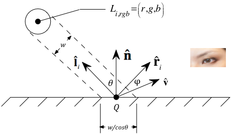
The basic geometry of reflection assumed by the Phong Empirical Local Lighting Model
Light is emitted from sources in an environment, and that light bounces all around the environment, generally illuminating all surfaces to some extent. In addition, some objects in an environment have surface and/or material properties that allow us to see reflections of other objects and/or see refracted images of objects behind them.

The effects mentioned above – multiple light reflections, reflected images of objects on the surfaces of others, and the ability to see through translucent objects – are generally called global lighting effects. In pipelined graphics engine architectures such as that present in OpenGL, such global effects are at best difficult to model in a general way. Various global approaches (e.g., ray tracing and radiosity) are typically used to simulate these effects. We will restrict ourselves to the study of local lighting models which explicitly do not attempt to simulate shadows (which are a side effect of how light scatters in an environment), reflections, and refraction.
Local models simulate the physics of light-surface interaction. A large number of local lighting models have been developed over the years, all based on geometric considerations along with various loose approximations to the underlying physics. The classical model used in pipelined graphics architectures (and in many ray tracers) is based on the Phong local lighting model. Other models that attempt to simulate more precisely the actual physics have been developed. While capable of producing extremely realistic results (see the figure on the right), they are considerably more computationally intensive and require a not insignificant amount of "tuning". Increasing GPU performance in recent years coupled with the fact that the shader stages are fully programmable makes it more reasonable to implement such advanced reflection models. Nevertheless, we will study only the classical Phong model since it is sufficiently complex for our purposes, easier to utilize, and produces perfectly good results for our purposes.
We can understand one aspect of the difference between empirical and physically-based models by reviewing something of the physics of electromagnetic radiation and color. Physical models attempt to sample a large number of reflected wavelengths; empirical models such as the Phong model we are about to study sample at just three wavelengths, corresponding roughly to blue, green, and red, respectively.
Creating a good lighting environment is required in order to get satisfying rendered results. It is also harder than you might think.
The value for c should generally be small, probably something like 0.1 ≤ c ≤ 0.2. It is also usually the same for all three channels; i.e., r = g = b = c.
The values used for c here indicate light source strength per color channel. They will be different for each of the (r, g, b) channels if you want to simulate colored light sources. Care must be taken with multiple light sources to try to avoid overflow of a color channel. An important part of good scene design is iterative adjustment of light source strengths to avoid this.
Specifying c0>0 protects you from cases where d is zero or close to it. Using c0=1, for example, is very common since that means in the limit as d→0, the attenuation approaches 1 (i.e., no attenuation).
We compute d in eye coordinates during the course of evaluating the lighting model. Why is this an issue? Suppose I compute dInEC=2. If the overall scene dimensions are, say, 20x20x20, I wouldn't want the light source to be attenuated nearly as much as I would if the scene dimensions were, say, 2x2x2. To as great an extent as possible, we would like to make our lighting model independent of the dimensions of any given scene. LDS coordinates provide such a system. If you review the projection matrices we derived, it should be clear that we can get a distance measure in LDS (and hence one that works regardless of overall scene dimensions) by computing and using dInLDS = ec_lds[0][0]*dInEC. However, most distances will be less than one, which would potentially impact the effectiveness of our attentuation. We could address that by essentially scaling so that distance becomes a percentage: dForAttenuation = ec_lds[0][0]*dInEC*100.0. Regardless of which d measure you use, tuning of the ci parameters will be needed.
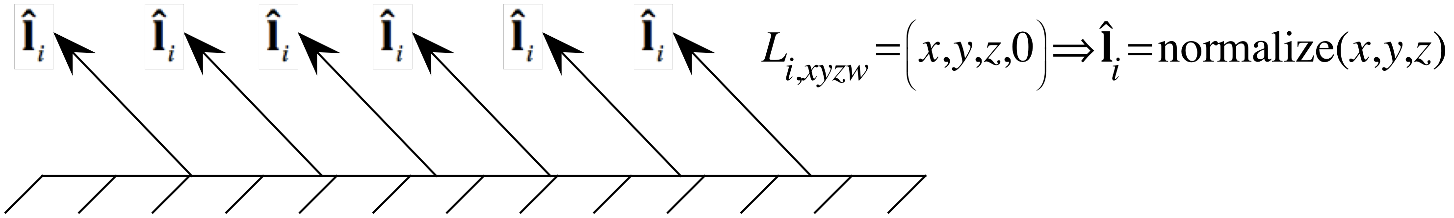
| Directional (e.g., sun, moon) | Positional (e.g.,lamps, ceiling lights) | Example Use | |
| Defined in Eye Coordinates? | (x, y, z, 0) | (x, y, z, 1) & attenuation specification | Viewer holding a flashlight |
| Defined in Model Coordinates? | (x, y, z, 0) | (x, y, z, 1) & attenuation specification | Almost everything else: sun, moon, lamp in a room, street light, … |
When modeling scenes from our everyday experience, we usually define light sources in the same coordinate system as the rest of our scene: model coordinates. The position of a lamp in a room is placed with respect to a table in the room. Even directions to sources like the sun and the moon should be specified in MC to avoid unrealistic effects during dynamic rotations.
The basic geometry of reflection assumed by the Phong Empirical Local Lighting Model
If the ith light source is defined in MC, the first step is to transform it to EC using the current mc_ec matrix. This can be done on the CPU before sending the data down, or on the GPU in the fragment shader.
There are two common ways to determine the unit vector towards the light source:

Decompose ![]() into its components parallel to and perpendicular to
into its components parallel to and perpendicular to
![]() .
Then
.
Then ![]() is (the parallel component - the perpendicular component):
is (the parallel component - the perpendicular component):
Classical Phong Local Lighting Model