 |
 |
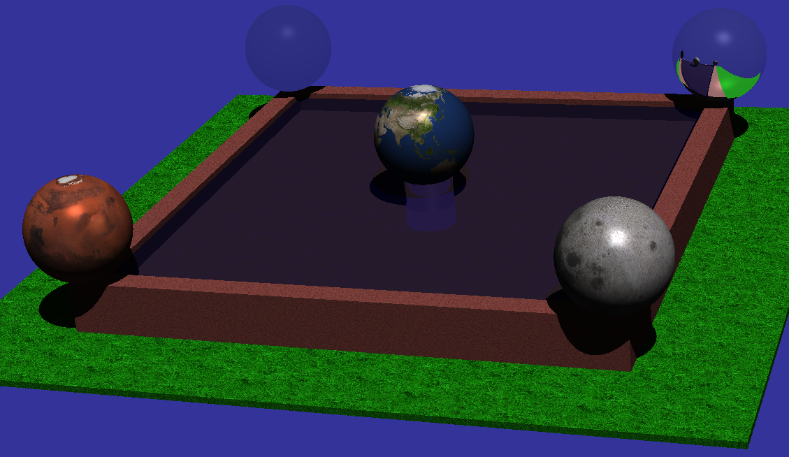 |
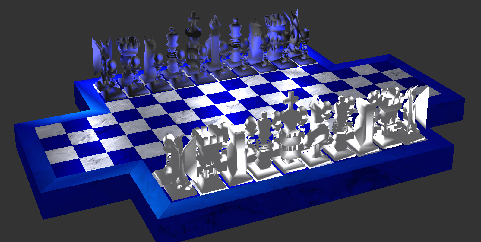
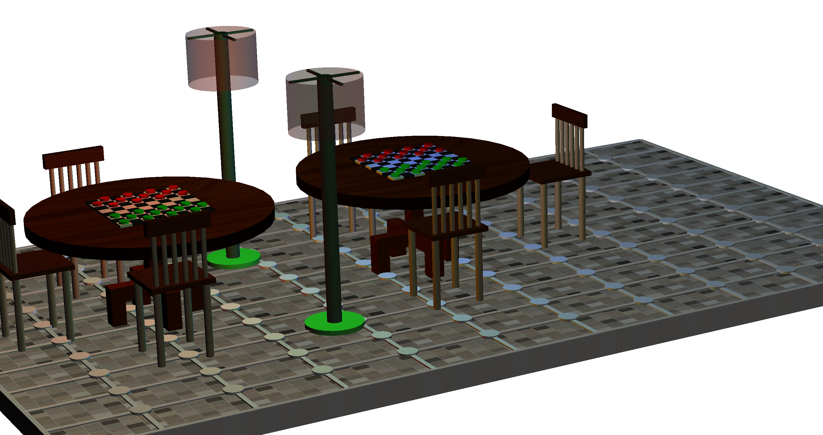
| Notice the refraction, shadows, and reflections in the scene above. It was rendered using a ray tracing algorithm implemented in a fragment shader. |
 |
 |
 |
 |
 |
 |
 |
 |
 |
 |
 |
 |
This course presents basic 2D and 3D interactive modeling and rendering using OpenGL and OpenGL's GPU shader language, GLSL. Shader-based OpenGL is an API whose design is based on a view of graphics programming in which modeling and rendering are cooperative undertakings between the CPU and the GPU. Graphics programs consist in part of C++ code running on the CPU and in part GLSL code running on the GPU.
The course covers basic 2D and 3D graphics concepts, interaction, and simple animation. Included are 3D modeling techniques (initially polygon-based, later curves and surfaces), viewing, and realistic lighting and shading models.
We focus on desktop applications using modern shader-based OpenGL and its C/C++ API. However, we will also discuss several very similar variants: OpenGL ES 2.0 (the version of OpenGL that runs on portable devices like Android and iOS platforms), JOGL (the Java binding to OpenGL for desktop applications that can be launched from web browsers using the Java Web Start mechanism), and WebGL (a variant of OpenGL ES 2.0 in which OpenGL programs are written in JavaScript and run entirely inside of web browsers).
From the beginning of the course, we will see how and why GPU programming has become of central importance to interactive graphics programming, how the design of the OpenGL API has evolved to enable real-time display and fully interactive manipulation of massive models (such as the lidar images below which can consist of tens of millions of points), and we will learn how to write sophisticated GLSL GPU shader programs.
In parallel with studying the structure and use of OpenGL and GLSL, we also study key general 3D modeling and rendering techniques (e.g., the roles played by points, vectors, and matrices; how matrices for specific purposes are constructed; and the pervasive use of piecewise linear approximation required to generate the models shown on this page).
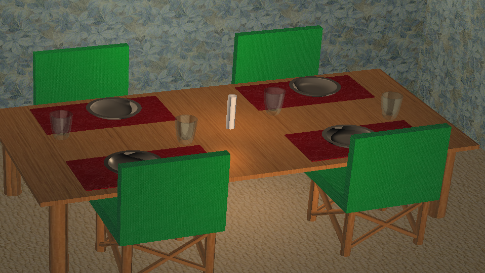
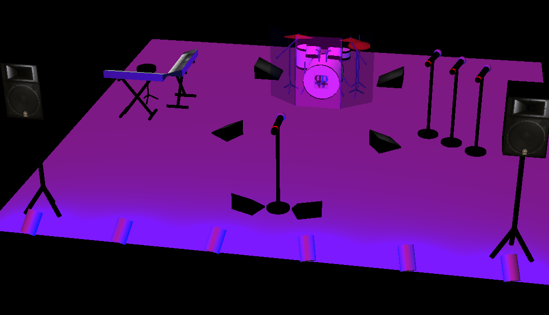
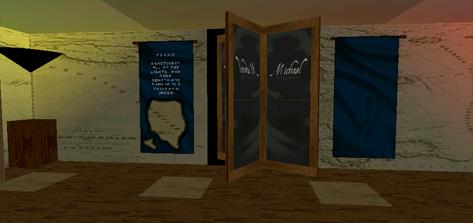
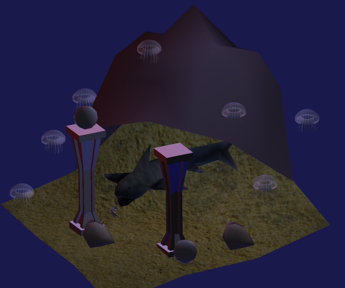
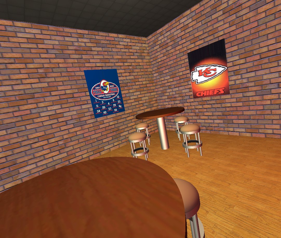
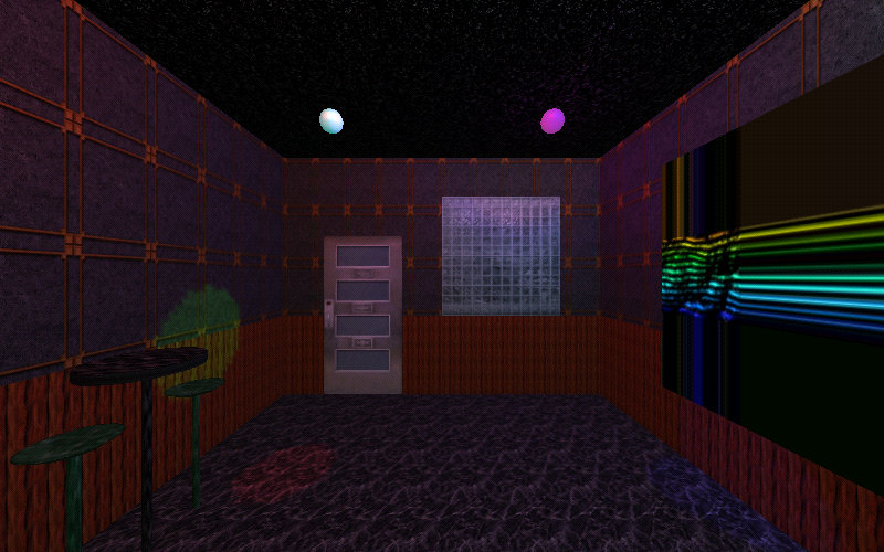
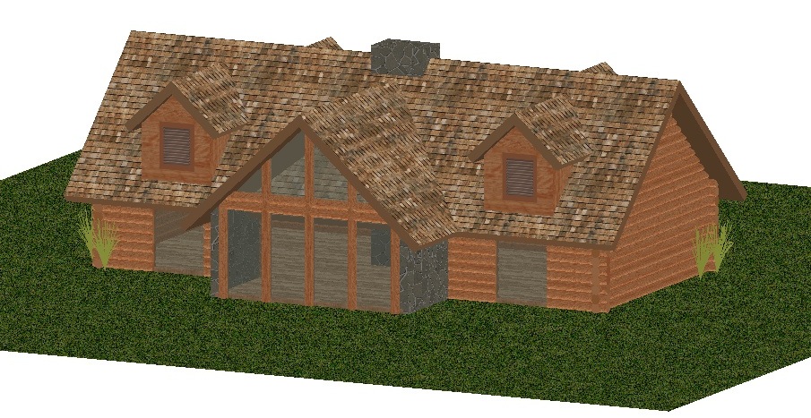
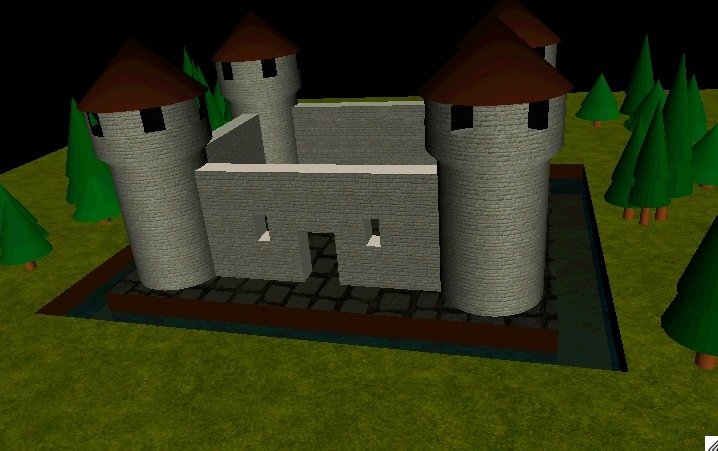
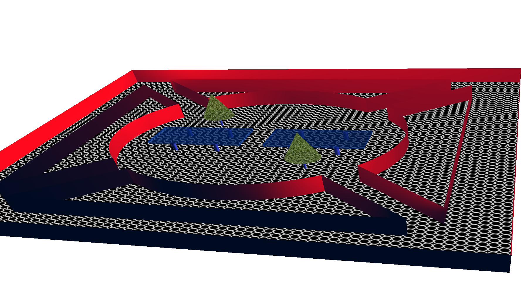
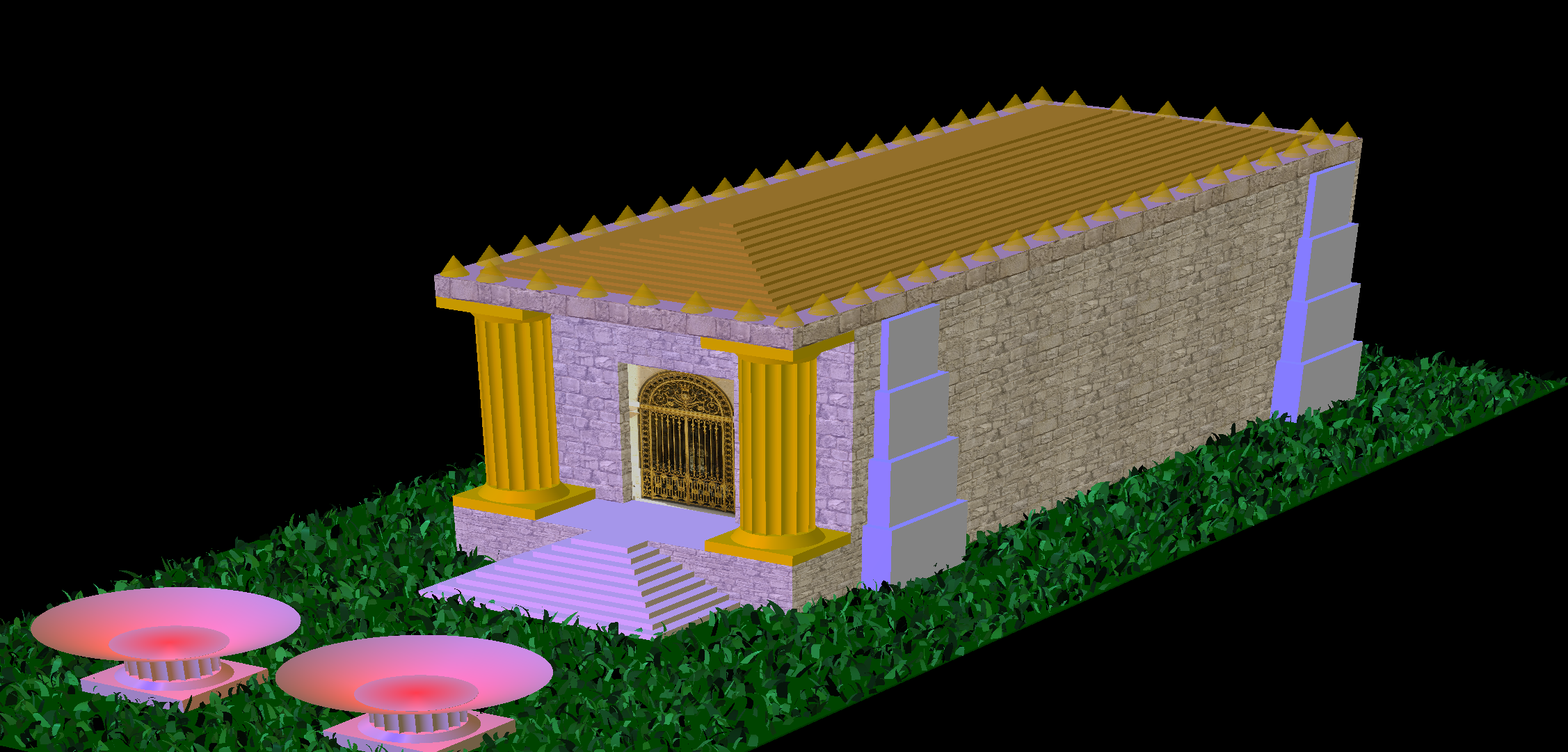
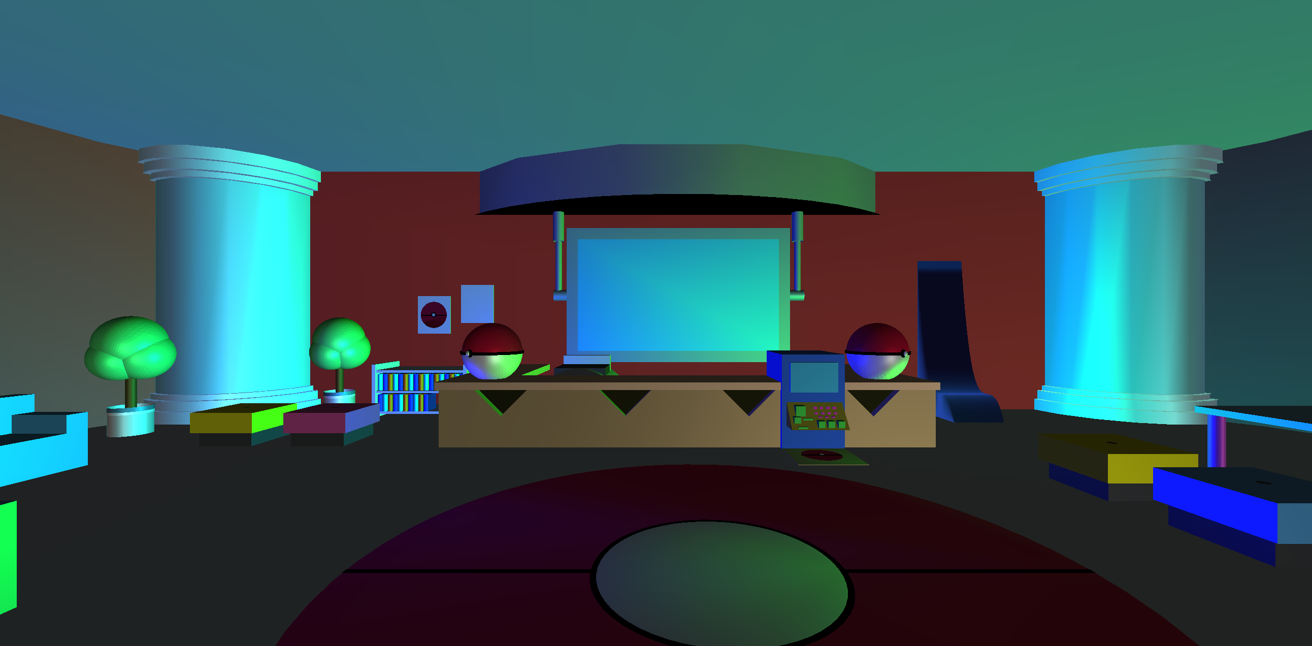
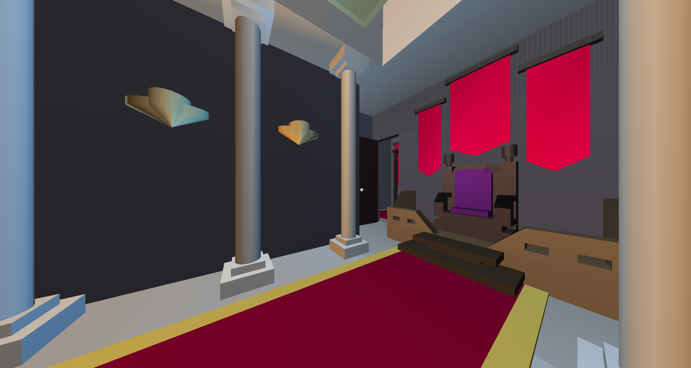
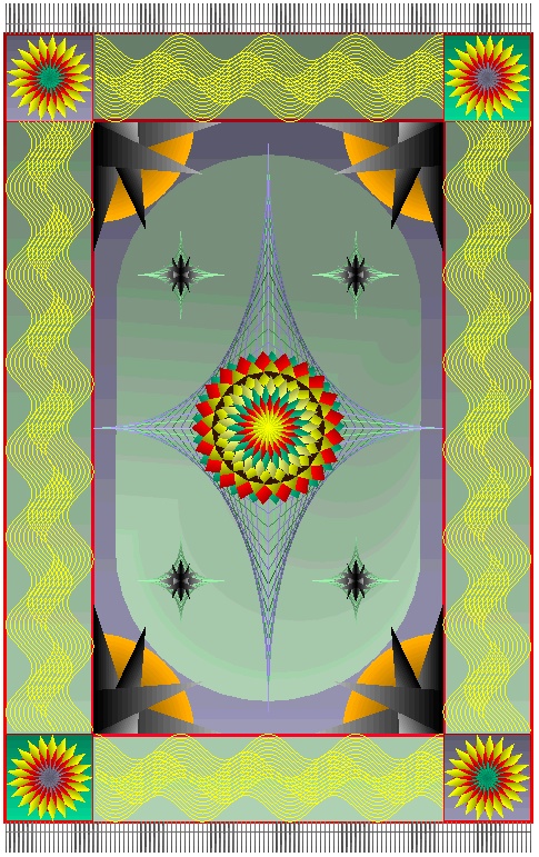
Except for the lidar images at the bottom, all scenes in images on this page were created and rendered by previous students in this course. Right click → "View Image" to see images at their actual captured resolution.
|
|
|
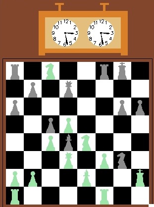
| Notice the refraction, shadows, and reflections in the scene above. It was rendered using a ray tracing algorithm implemented in a fragment shader. |
|
|
|
|
|
|
|
|
|
|
|
|
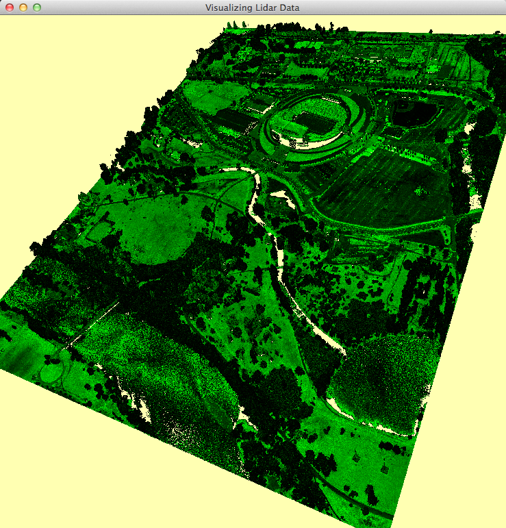 11 million lidar points colored by pulse return intensity |
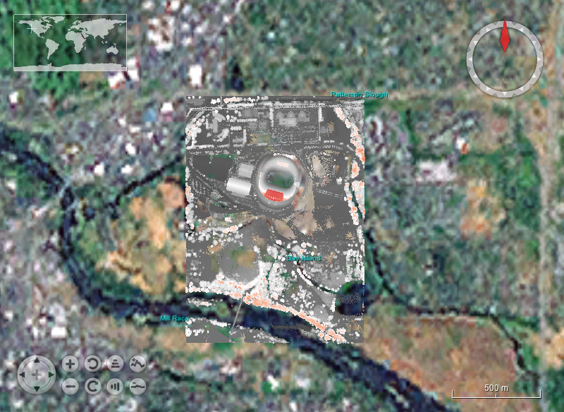 The same set of points georeferenced, colored based on elevation, and drawn in NASA World Wind |
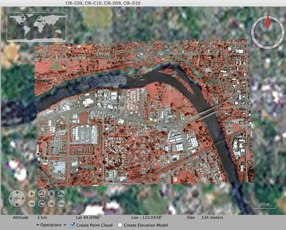
Approximately 15 million lidar data points, colored using orthorectified areal infrared imagery.