Curves & Surfaces:

Purpose and Context

Very simply stated, geometry modeling is all about representing and manipulating shapes. Shape taxonomies can be constructed in many different ways, depending on your context, point of view, or application. One starting point that is appropriate for this course is based on whether we are trying to represent (portions of) the boundary or external "skin" of an object versus trying to completely characterize how its shape and properties vary throughout its volumetric extent. The former leads to the study of curves and surfaces, and the latter leads to the study of solid modeling.

This high level overview focuses on the former. It starts by reviewing some common applications of curve and surface modeling, and then moves on to mathematical representations.

Applications

Model Design Relatively simple, e.g.: Stapler, pen, mug Telephone and other shapes with smooth "transition" surfaces Bottles (shampoo, perfume, lotion, etc.), shoes Teapots More complex, e.g.: humans, animals, and other organic shapes cars body (aesthetics, aerodynamics) engine and its component parts (packaging & fit, weight, durability) fuel tank (maximize volume, fit empty space, tilt test requirements) airplanes fuselage, wings (aerodynamics) wiring, components (routing, packaging) interior spaces (human comfort, ventilation) Bioinformatics Curve fitting has been used during some types of gene sequencing analysis. Surfaces arise in several contexts (molecular surfaces, solvent-accessible surfaces, and others). Font design Animation and movie production (e.g., animation paths, articulated characters)

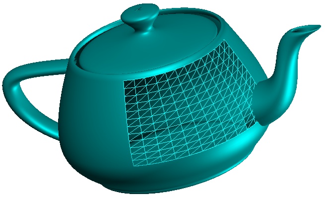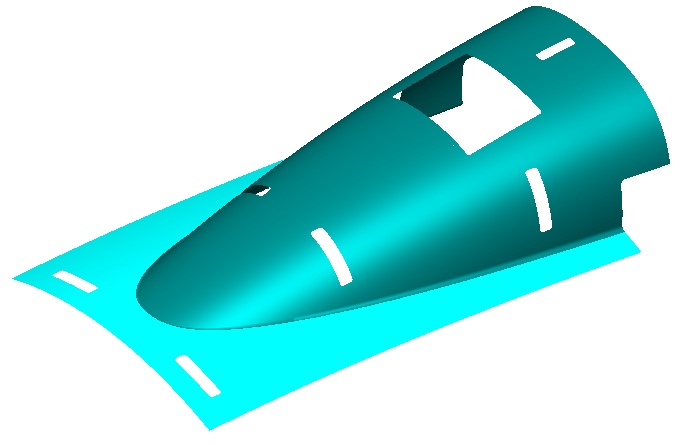On Mathematical Representations

Intrinsic Equations

The shape of a curve is an intrinsic property that can be uniquely and completely described by two scalar parametric equations, one describing its curvature (κ) and the other its torsion (τ). Both are described as functions of arc length along the curve: κ=f(s) and τ=g(s). At each point on the curve, we can define a plane (called the osculating plane) in which the curve locally lies (e.g., its tangent vector lies in this plane). The quantity κ is a measure of how the tangent vector is changing in the plane, and τ is a measure of how much the curve is twisting out of the osculating plane. Curvature is sometimes written as κ=1/ρ, where ρ is the radius of a circle in the osculating plane whose tangent and curvature exactly match that of the curve at the point.

Algebraic (Explicit and Implicit) and Parametric Equations

Many important theoretical aspects of curves (e.g., the Fundamental Theorem of Curves) derive from a study of intrinsic equations. We shall not consider them further at this point, however. Instead we turn our attention to representations commonly used in computer-based implementations of design and analysis operations. For such purposes, curves and surfaces are normally written either in algebraic or parametric form. Both describe not only the shape of the curve, but also its exact position and orientation with respect to some given reference coordinate system.

Algebraic representations can be one of two types. Implicit algebraic representations describe a curve or surface as the zero set of some function. For example, a planar curve in the xy plane would be described as { (x,y) | f(x,y) = 0 }. Similarly, a surface would be described as { (x,y, z) | f(x,y, z) = 0 }.

Explicit algebraic representations describe one coordinate of a curve or surface as an explicit function of the others. An explicit representation of a 2D curve would be represented as y = f(x). An explicit representation of a surface could be represented as z = f(x, y). Height surfaces in GIS application domains are one very common example.

Parametric representations introduce one (for curves) or two (for surfaces) independent parameters and are a prescriptive form. That is, they describe how to generate an ordered sequence of points along the curve or surface. We describe them as a mapping from the 1D or 2D parametric domain into the 2D or 3D affine space in which the curve or surface lies.

The general form for algebraic and parametric representations of curves and surfaces is summarized in the table below.

DERIVATIVES, TANGENTS, AND NORMAL VECTORS

The implicit and parametric forms as reviewed above describe the points on the curves and surfaces themselves. Derivatives can be used to obtain vectors tangent to and perpendicular to given curves and surfaces. Specifically:

• The gradient operator – ∇ = (∂/∂x, ∂/∂y) in 2D, or ∇ = (∂/∂x, ∂/∂y, ∂/∂z) in 3D – can be used to obtain vectors perpendicular to curves and surfaces represented with implicit algebraic equations.
• Ordinary derivatives are used to compute vectors tangent to curves represented with parametric polynomial equations.
• Partial derivatives are used to compute vectors tangent to surfaces represented with parametric polynomial equations.
• A vector perpendicular to a parametric curve or surface can be computed by first finding the tangent(s) and then using a cross product.

VECTOR GEOMETRIC NOTATION

Implicit and parametric representations can quickly become unwieldy if we continue to focus on their x, y, and z components. Vector geometric notation can keep things much more manageable. As a first simple example, rather than writing the equation of a sphere componentwise as:

we assume our unknown variable X = (x, y, z), our center C = (C_x, C_y, C_z), and we write:

Similarly, instead of writing the parametric equation of a circle in some plane spanned by mutually perpendicular unit vectors u and v as:

we write:

POLYNOMIALS VERSUS OTHER FUNCTIONS

We will primarily restrict ourselves to the study of freeform curves and surfaces that can be represented by functions that are polynomial in the variables (e.g., x, y, and z; s and t). However we also frequently see trigonometric functions. If you are generating points around a circle or an ellipse (or generating points on a surface like a sphere or cylinder), trigonometric functions are most likely your best choice.

On the other hand, polynomials are nice for several reasons including:

• The range of shapes they can produce is very rich.
• Their mathematical and computational properties (e.g., differentiability and computational efficiency) are good.
• Boatloads of algorithms are known for important tasks like interpolation, approximation, intersection, and many others.
• Important theoretical results (e.g., Bezout's Theorem) apply to curves and surfaces that can be represented using polynomial functions.

Parametric curves represented using trigonometric functions can be re-represented as rational polynomials: i.e., the quotient of two ordinary polynomials. As long as we agree to a few occasional bookkeeping shenanigans, curves such as our circle can be parameterized as:

Considering this representation, we can generalize our description of the mapping involved in parametric representations: rational polynomial curves and surfaces can be described as a mapping from the 1D or 2D parametric domain into the 3D or 4D projective space in which the affine space containing the curve or surface is embedded. Specifically:

where

Conversion of an arbitrary trigonometric parameterization into a rational polynomial parameterization is accomplished using a change of variable approach. Specifically, the following substitutions as introduced above are straightforward to derive: