A Very Brief Introduction to Parametric Curves & Surfaces

Earlier this semester we saw how we could generate piecewise linear approximations of circles using one of the following parameterizations:

Simple 2D circle with origin (c_x, c_y) and radius, r:
C(θ) = (c_x + r*cos(θ), c_y + r*sin(θ))
A 3D circle in arbitrary position and orientation: center, C, "local x-axis": u, "local y-axis": v, and radius, r:
C(θ) = C + r * (cos(θ)u + sin(θ)v)
where
- C is a point: (C_x, C_y, C_z)
- u and v are unit vectors perpendicular to each other: (dx, dy, dz)
This is clearly a generalization of the "simple 2D circle" parameterization since that circle can be generated using C = (c_x, c_y, 0), u = (1, 0, 0), and v = (0, 1, 0).

While curves based on conic sections are often parameterized using trigonometric functions like this, it is far more common to use polynomials of degree n when modeling other types of curves. We also typically use a different parameter variable (e.g., t, u, v, etc.) instead of θ since the parameter no longer refers to an angle, rather to some sort of distance measure along the curve. In the simplest case, this would look like:

P(t) = a₀ + a₁t + a₂t² + … + a_ntⁿ

where:

a₀ is a point: (x₀, y₀, z₀)
a_i, 1 ≤ i ≤ n, is a vector: (dx_i, dy_i, dz_i)

This form is not at all common as a general modeling representation because it is far too difficult to determine values for the various a_k to achieve a desired shape. Even if we were given a set of a_k that produced a shape close to what we wanted, it would be unreasonably complex to determine how to adjust the a_k to tweak the shape in some particular fashion.

The form shown above is called the Power Basis representation of the curve. Polynomials of degree n form a vector space. The "polynomial vectors" of the Power Basis, namely (1, t, t², …, tⁿ), span this space, which means that any polynomial of degree n can be written as a linear combination of these quantities. (Nothing new there; you already knew that.)

There are many other families of (n + 1) polynomials that also span the space of degree n polynomials. One common one (that you have no doubt encountered in statistics applications) is the Bernstein Basis:

Like the Power Basis, any polynomial of degree n can be written as a linear combination of the B_{i, n}. Unlike the Power Basis, the Bernstein basis has a very nice property:

This means we can use them to form a functional Barycentric combination of (n + 1) points P₀, P₁, …, P_n:

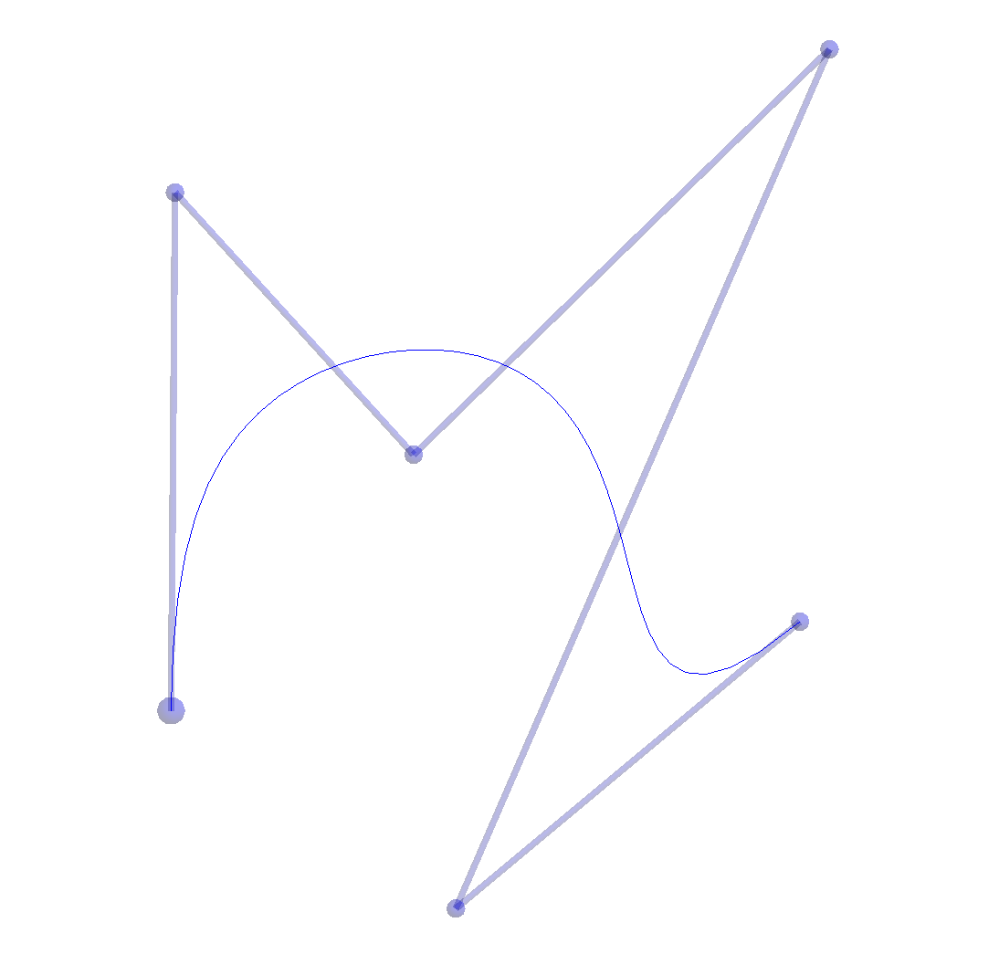
Why would we want to? For starters, C(t) will be a well-defined point for any value of t. (Right?) Moreover, it turns out that the set of points that result define a continuous curve with some very desirable properties. When drawn from t=0 to t=1, the curve starts at P₀; it ends at P_n; and its shape follows that of the rest of the points in a very intuitive way. This means initial curve construction as well as subsequent modification can be extremely intuitive.

Note also the fact that on the interval 0 ≤ t ≤ 1, all of the B_{i, n}(t) are non-negative. Hence, the summation defining C(t) is a convex combination on this interval. Recall that any point, Q, formed as a convex combination of a set of points, P_i, will lie inside the convex hull of the P_i. This means the entire curve on 0 ≤ t ≤ 1 will lie inside the convex hull of the P_i, a property that also contributes to this form being particularly well-suited for interactive shape design.

A curve defined in this way is shown on the right and is called a Bezier Curve.

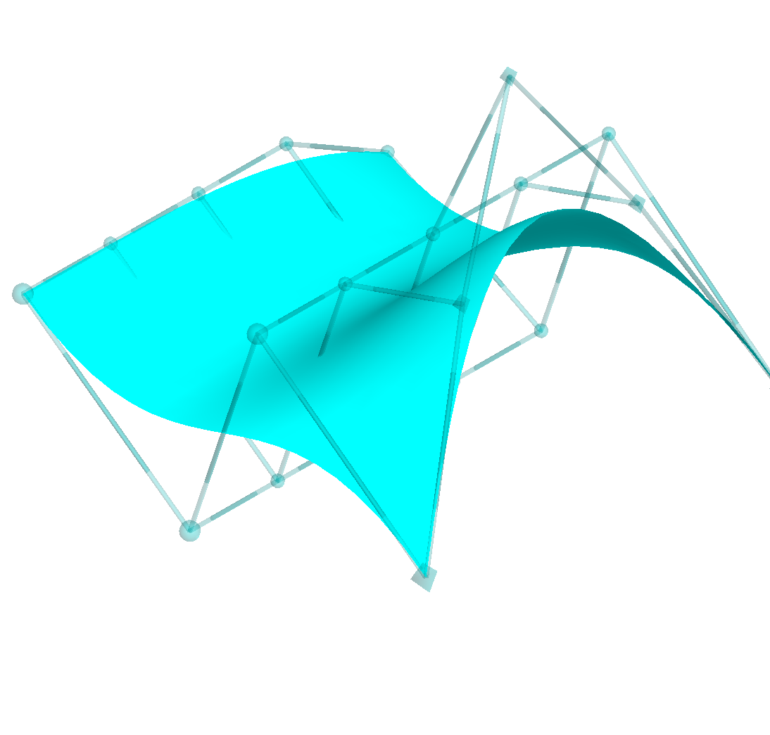
It turns out we can define a Bezier Surface in a similar way:

An example of such a surface with n=4 and m=3 is shown below.